
|
VLookup Function Home Microsoft Excel Microsoft Access custom Reports SQL Server Visual Basic |
The VLookup function is a powerful tool in Excel. VLookup is a function that looks for a match
in a data table, and returns a selected value. The HLookup function works similarly; where the
VLookup function queries down a set of rows, the HLookup function queries across a series of
columns. Since database like tables are almost always arranged where each row represents a
record, and each column represents a field, the VLookup funciton is much more common.
While the VLookup function is described here, the HLookup function uses the same arguments, with
the opposite orientation. The syntax of the VLookup funciton is: =VLookup(lookup value, table range, column number[, Range lookup) The arguments (data passed to the lookup function for it to process) are described as follows:
To demonstrate the VLookup function, suppose you have a list of items on one sheet, and a list of prices on another sheet. The Items sheet might look like this: 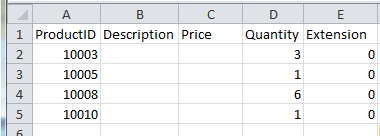 Let's say you have a different sheet in the same workbook that has the prices: 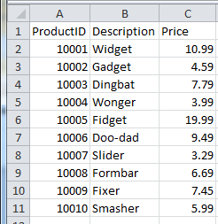 In this example, you would want to put the description in Column B, and the price in Column C for each row. In cell B2, you would type =VLookup( to start the function. The lookup value is in cell A2, the item number. Continue typing A2 (or point at cell A2), then type the comma. For the lookup table, it is easier (but not required) to have the data on a different sheet in the workbook. If your lookup table is on a second sheet, click the tab for that sheet, then select the data. The data range must have as its leftmost column where the data to be found is (the item number in this case), and must include the column that has the desired value in it. It can include extra columns, and the selection can be either the data area or the entire columns containing the data. If you select a range, you will invariably want to make the range an absolute reference by touching the F4 key, otherwise when you copy your lookup function, the cell references will change. Type a comma to indicate the end of the second argument for the VLookup function. For the example, the formula bar should how show =VLookup(A2,Sheet2!$A$2:$C$11, The third argument is the column number. Start with the leftmost column of the lookup table, and count columns starting at 1. For the first VLookup function, where we want the description, the Description is in the second column of the lookup table. Type 2 for the column number. The fourth argument for the VLookup function is optional, but it is important to how the VLookup function works. If the Range Lookup argument is not supplied, True is the default. This means that Excel will return the greatest value that is less than the lookup value if an exact match does not exist. If you specify true, or omit the argument, the list must be sorted to work reliably. Particularly where an exact match is desired, and an error would be desirable if there were no exact match, specify False. This argument should only be omitted where it is desirable to find approximate matches. Thus, continue the VLookup with the FALSE argument. Type the closing parenthesis ), touch the ENTER key, and the VLookup is complete: 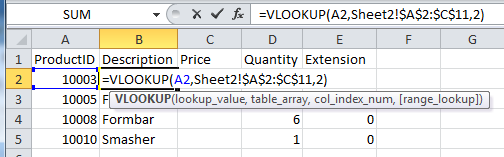 For expert help with the VLookup function, or other advanced Excel features and functions, call us at (303) 403-0386 or e-mail us. |
Copyright 2012 Front Range Data Management Services